Saturday, September 15, 2018

MEDICAL PHYSICS

Tags

Related image

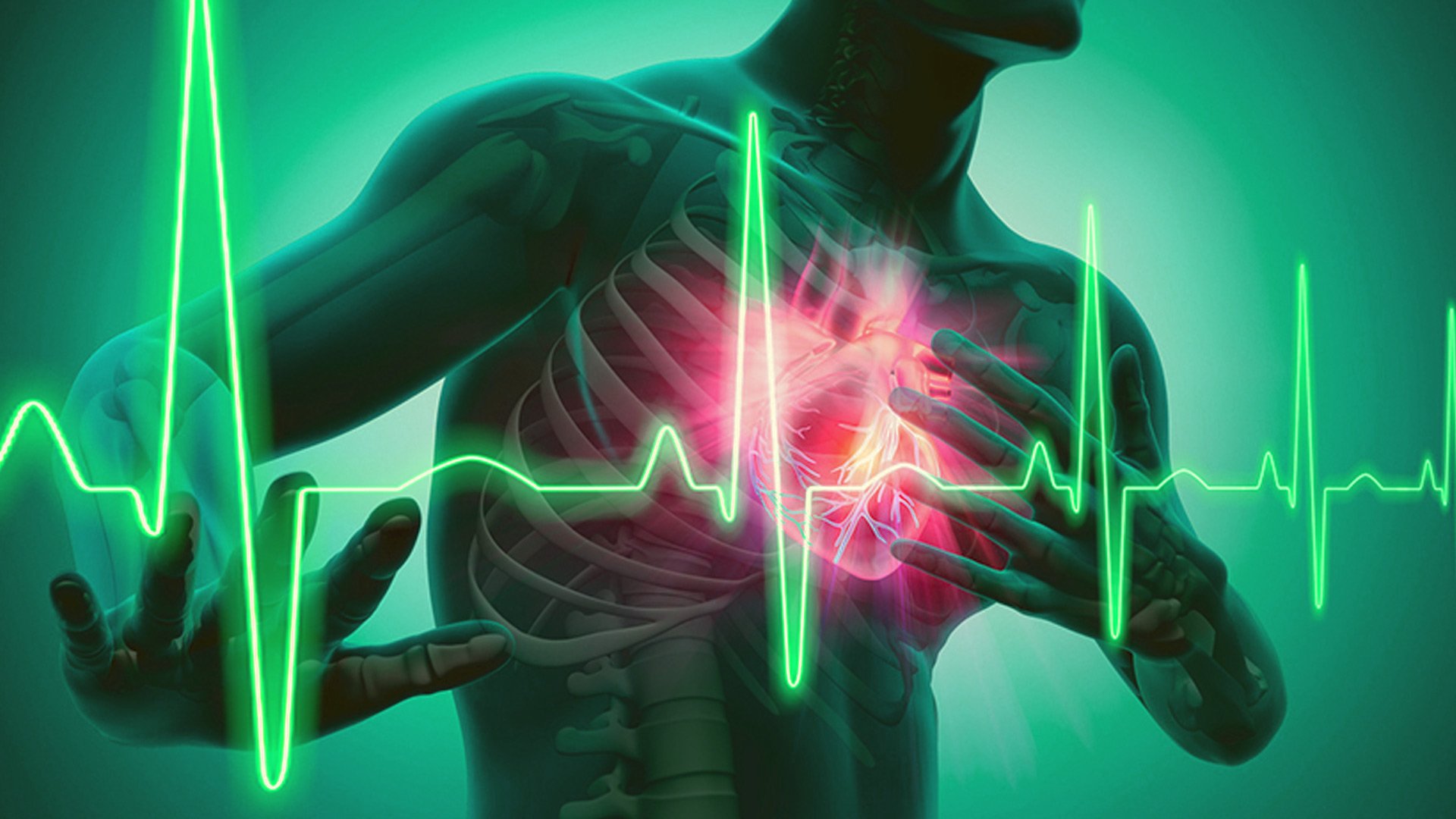
 Cardiac stimulation: fibrillation


    Electromedical equipment is a possible source of hazard to the patient. In many cases the patient is directly connected to the equipment so that in cases of a fault electrical current may flow through the patient. The response of the body to low-frequency alternating current depends on the frequency and the current density. Low-frequency current (up to 1 kHz) which includes the main commercial supply frequencies (50 Hz and 60 Hz) can cause: prolonged tetanic contraction of skeletal and respiratory muscles; arrest of respiration by interference with the muscles that control breathing; heart failure due to ventricular fibrillation (VF). In calculating current through the body, it is useful to model the body as a resistor network. The skin can have a resistance as high as 1 M (dry skin) falling to 1 k (damp skin). Internally, the body resistance is about 50. Internal conduction occurs mainly through muscular pathways. Ohm’s law can be used to calculate the current. For example, for a person with damp skin touching both terminals of a constant voltage 240 V source (or one terminal and ground in the case of mains supply), the current would be given by I = V /R = 240/2050 = 117 mA, which is enough to cause ventricular fibrillation (VF).

Indirect cardiac stimulation


   Most accidental contact with electrical circuits occurs via the skin surface. The threshold of current perception is about 1 mA, when a tingling sensation is felt. At 5 mA, sensory nerves are stimulated. Above 10 mA, it becomes increasingly difficult to let go of the conductor due to muscle contraction. At high levels the sustained muscle contraction prevents the victim from releasing their grip. When the surface current reaches about 70–100 mA the co-ordinated electrical control of the heart may be affected, causing ventricular fibrillation (VF).

The fibrillation may continue after the current is removed and will result in death after a few minutes if it persists. Larger currents of several amperes may cause respiratory paralysis and burns due to heating effects. The whole of the myocardium contracts at once producing cardiac arrest. However, when the current stops the heart will not fibrillate, but will return to normal co-ordinated pumping. This is due to the cells in the heart all being in an identical state of contraction. This is the principle behind the defibrillator where the application of a large current for a very short time will stop ventricular fibrillation.

 The VF threshold varies in a similar way; currents well above 1 kHz, as used in diathermy, do not stimulate muscles and the heating effect becomes dominant. IEC 601-1 limits the AC leakage current from equipment in normal use to 0.1 mA.

Direct cardiac stimulation


    Currents of less than 1 mA, although below the level of perception for surface currents, are very dangerous if they pass internally in the body in the region of the heart. They can result in ventricular fibrillation and loss of pumping action of the heart.

Currents can enter the heart via pacemaker leads or via fluid-filled catheters used for pressure monitoring. The smallest current that can produce VF, when applied directly to the ventricles, is about 50 μA. British Standard BS5724 limits the normal leakage current from equipment in the vicinity of an electrically susceptible patient (i.e. one with a direct connection to the heart) to 10 μA, rising to 50 μA for a single-fault condition.

Note that the 0.5 mA limit for leakage currents from normal equipment is below the threshold of perception. but above the VF threshold for currents applied to the heart. Percentage of adult males who can ‘let go’ as a function of frequency and current.

Ventricular fibrillation VF occurs when heart muscle cells coming out of their refractory period are electrically stimulated by the fibrillating current and depolarize, while at the same instant other cells, still being in the refractory period, are unaffected. The cells depolarizing at the wrong time propagate an impulse causing other cells to depolarize at the wrong time. Thus, the timing is upset and the heart muscles contract in an unco-ordinated fashion. The heart is unable to pump blood and the blood pressure drops. Death will occur in a few minutes due to lack of oxygen supply to the brain. To stop fibrillation, the heart cells must be electrically co-ordinated by use of a defibrillator.

The threshold at which VF occurs is dependent on the current density through the heart, regardless of
the actual current. As the cross-sectional area of a catheter decreases, a given current will produce increasing current densities, and so the VF threshold will decrease.

HIGHER FREQUENCIES: >100 kHz


 Surgical diathermy/electrosurgery


Surgical diathermy/electrosurgery is a technique that is widely used by surgeons. The technique uses an electric arc struck between a needle and tissue in order to cut the tissue. The arc, which has a temperature in excess of 1000 ◦ C, disrupts the cells in front of the needle so that the tissue parts as if cut by a knife; with suitable conditions of electric power the cut surfaces do not bleed at all. If blood vessels are cut these may continue to bleed and current has to be applied specifically to the cut ends of the vessel by applying a blunt electrode and passing the diathermy current for a second, or two or by gripping the end of the bleeding vessel with artery forceps and passing diathermy current from the forceps into the tissue until the blood has coagulated sufficiently to stop any further bleeding. Diathermy can therefore be used both for cutting and coagulation.

The current from the ‘live’ or ‘active’ electrode spreads out in the patient’s body to travel to the
‘indifferent’, ‘plate’ or ‘patient’ electrode which is a large electrode in intimate contact with the patient’s body. Only at points of high current density, i.e. in the immediate vicinity of the active electrode, will coagulation take place; further away the current density is too small to have any effect. Although electricity from the mains supply would be capable of stopping bleeding, the amount of
current needed (a few hundred milliamperes) would cause such intense muscle activation that it would be impossible for the surgeon to work and would be likely to cause the patient’s heart to stop. The current used must therefore be at a sufficiently high frequency that it can pass through tissue without activating the muscles.

Diathermy equipment


Diathermy machines operate in the radio-frequency (RF) range of the spectrum, typically 0.4–3 MHz.
Diathermy works by heating body tissues to very high temperatures. The current densities at the active electrode can be 10 A cm −2 . The total power input can be about 200 W. The power density in the vicinity of the cutting edge can be thousands of W cm −3 , falling to a small fraction of a W cm −3 a few centimetres from the cutting edge. The massive temperature rises at the edge (theoretically thousands of ◦ C) cause the tissue fluids to boil in a fraction of a second. The cutting is a result of rupture of the cells.

An RF current follows the path of least resistance to ground. This would normally be via the plate (also called dispersive) electrode. However, if the patient is connected to the ground via the table or any attached leads from monitoring equipment, the current will flow out through these. The current density will be high at these points of contact, and will result in surface burns (50 mA cm −2 will cause reddening of the skin; 150 mA cm −2 will cause burns). Even if the operating table is insulated from earth, it can form a capacitor with the surrounding metal of the operating theatre due to its size, allowing current to flow. Inductive or capacitive coupling can also be formed between electrical leads, providing other routes to ground.

 Heating effects


If the whole body or even a major part of the body is exposed to an intense electromagnetic field then the heating produced might be significant. The body normally maintains a stable deep-body temperature within relatively narrow limits (37.4 ± 1 ◦ C) even though the environmental temperature may fluctuate widely. The normal minimal metabolic rate for a resting human is about 45 W m −2 (4.5 mW cm −2 ), which for an average surface area of 1.8 m 2 gives a rate of 81 W for a human body. Blood perfusion has an important role in maintaining deep-body temperature. The rate of blood flow in the skin is an important factor influencing the internal thermal conductance of the body: the higher the blood flow and hence, the thermal conductance, the greater is the rate of transfer of metabolic heat from the tissues to the skin for a given temperature difference.

   Blood flowing through veins just below the skin plays an important part in controlling heat transfer. Studies have shown that the thermal gradient from within the patient to the skin surface covers a large range and gradients of 0.05–0.5 ◦ C mm −1 have been measured. It has been shown that the effect of radiation emanating from beneath the skin surface is very small. However, surface temperatures will be affected by vessels carrying blood at a temperature higher or lower than the surrounding tissue provided the vessels are within a few millimetres of the skin surface. Exposure to electromagnetic (EM) fields can cause significant changes in total body temperature. Some of the fields quoted in table 8.3 are given in volts per metre. We can calculate what power dissipation this might cause if we make simplifying assumptions, which represents a body which is 30 cm in diameter and 1 m long (L). We will assume a resistivity (ρ) of 5m for the tissue. The resistance (R) between the top and bottom will be given by ρL/A where A is the cross-sectional area. R = 70.7 For a field of 1 V m −1 (in the tissue) the current will be 14.1 mA. The power dissipated is 14.1 mW which is negligible compared to the basal metabolic rate. applied fielddiameter 30 cm length 100 cm resistivity assumed to be 5 ohm metre. The body modelled as a cylinder of tissue. For a field of 1 kV m −1 , the current will be 14.1 A and the power 14.1 kW, which is very significant.

  The power density is 20 W cm −2 over the input surface or 200 mW cm −3 over the whole volume.
In the above case we assumed that the quoted field density was the volts per metre produced in tissue.
However, in many cases the field is quoted as volts per metre in air. There is a large difference between these two cases. A field of 100 V m −1 in air may only give rise to a field of 10 −5 V m −1 in tissue.

ULTRAVIOLET


We now come to the border between ionizing and non-ionizing radiation. Ultraviolet radiation is part of the electromagnetic spectrum and lies between the visible and the x-ray regions. It is normally divided into three wavelength ranges. These define UV-A, UV-B and UV-C by wavelength.
A 315–400 nm
B 280–315 nm
C 100–280 nm

 The sun provides ultraviolet (mainly UV-A and UV-B) as well as visible radiation. Total solar irradiance is about 900 W m −2 at sea level, but only a small part of this is at ultraviolet wavelengths. Nonetheless there is sufficient UV to cause sunburn. The early effects of sunburn are pain, erythema, swelling and tanning. Chronic effects include skin hyperplasia, photoaging and pseudoporphyria. It has also been linked to the development of squamous cell carcinoma of the skin. Histologically there is subdermal oedema and other changes.

Of the early effects UV-A produces a peak biological effect after about 72 h, whereas UV-B peaks at
12–24 h. The effects depend upon skin type. The measurement of ultraviolet radiation Exposure to UV can be assessed by measuring the erythemal response of skin or by noting the effect on micro-organisms. There are various chemical techniques for measuring UV but it is most common to use
physics-based techniques. These include the use of photodiodes, photovoltaic cells, fluorescence detectors and thermoluminescent detectors such as lithium fluoride. Therapy with ultraviolet radiation Ultraviolet radiation is used in medicine to treat skin diseases and to relieve certain forms of itching. The UV radiation may be administered on its own or in conjunction with photoactive drugs, either applied directly to the skin or taken systemically.

The most common application of UV in treatment is psolaren ultraviolet A (PUVA). This has been
used extensively since the 1970s for the treatment of psoriasis and some other skin disorders. It involves the combination of the photoactive drug psoralen, with long-wave ultraviolet radiation (UV-A) to produce a beneficial effect. Psoralen photochemotherapy has been used to treat many skin diseases, although its principal success has been in the management of psoriasis. The mechanism of the treatment is thought to be that psoralens bind to DNA in the presence of UV-A, resulting in a transient inhibition of DNA synthesis and cell division. 8-methoxypsolaren and UV-A are used to stop epithelial cell proliferation. There can be side effects and so the dose of UV-A has to be controlled. Patch testing is often carried out in order to establish what dose will cause erythema. This minimum erythema dose (MED) can be used to determine the dose used during PUVA therapy.
In PUVA the psoralens may be applied to the skin directly or taken as tablets. If the psoriasis is
generalized, whole-body exposure is given in an irradiation cabinet. Typical intensities used are 10 mW cm −2 , i.e. 100 W m −2 . The UV-A dose per treatment session is generally in the range 1–10 J cm −2 . Treatment is given several times weekly until the psoriasis clears. The total time taken for this to occur will obviously vary considerably from one patient to another, and in some cases complete clearing of the lesions is never achieved. PUVA therapy is not a cure for psoriasis and repeated therapy is often needed to prevent relapse.

Friday, September 14, 2018

NON-IONISED ELECTROMAGNETIC RADIATION

Tags
Image result for the impedance as the function of frequency of two electrodes placed in the abdomen


NON-IONIZING ELECTROMAGNETIC RADIATION: TISSUE ABSORPTION AND SAFETY ISSUES


INTRODUCTION AND OBJECTIVES

An understanding of the interaction of electromagnetic radiation with tissue is important for many reasons, apart from its intrinsic interest. It underpins many imaging techniques, and it is essential to an understanding of the detection of electrical events within the body, and the effect of externally applied electric currents. In this text we assume that you have a basic understanding of electrostatics and electrodynamics, and we deal with the applications in other chapters. Our concern here is to provide the linking material between the underlying theory and the application, by concentrating on the relationship between electromagnetic fields and tissue. This is a complex subject, and our present state of knowledge is not sufficient for us to be able to provide a detailed model of the interaction with any specific tissue, even in the form of a statistical model.

We have also limited the frequency range to <10 16="" frequencies="" higher="" hz="" i.e.="" ionizing="" p="" radiation="" radio="" to="" ultraviolet.="" waves="">Some of the questions we will consider are
   Does tissue conduct electricity in the same way as a metal?
   Does tissue have both resistive and capacitive components?
   Do the electrical properties of tissue depend upon the frequency of electromagnetic radiation?
   Can any relatively simple models be used to describe the electrical properties of tissue?
   What biological effects might we predict will occur?
   When you have finished this chapter, you should be aware of
   The main biological effects of low-frequency electric fields.
   How tissue electrical properties change with frequency.
   The main biological effects of high-frequency fields such as IR and UV.
   How surgical diathermy/electrosurgery works Some of the safety issues involved in the use of electromedical equipment.

 There is some mathematics in this text,  These two sections assume some knowledge of the theory of dielectrics. However, the rest should be understandable to all of our readers. The purpose of including the first two sections is to give a theoretical basis for understanding the rest of the text which covers the practical problems of tissue interactions with electromagnetic fields. If our understanding of these interactions is to be quantitative then we need to have a theoretical baseline.


TISSUE AS A LEAKY DIELECTRIC

If two electrodes are placed over the abdomen and the electrical impedance is measured between them over a wide range of frequencies then the results obtained might be as shown in figure (1)


figure(1)
Image result for the impedance as the function of frequency of two electrodes placed in the abdomen


The results will depend somewhat upon the type and size of electrodes, particularly at the lowest frequencies, and exactly where the electrodes are placed. However, the result is mainly a function of the tissue properties. The impedance always drops with increasing frequency. This chapter is concerned first with trying to explain why tissue impedance changes with frequency in this way. It is an important question because unless we understand why tissue has characteristic electrical properties then we will not be able to understand how electromagnetic fields might affect us. We will start in this section by considering tissue as a lossy dielectric and then look at possible biological interactions with electromagnetic fields in later sections.

    We are familiar with the concept of conductors, which have free charge carriers, and of insulators,
which have dielectric properties as a result of the movement of bound charges under the influence of an applied electric field. Common sense tells us that an insulator cannot also be a conductor. Tissues though contain both free and bound charges, and thus exhibit simultaneously the properties of a conductor and a dielectric. If we consider tissue as a conductor, we have to include a term in the conductivity to account for the redistribution of bound charges in the dielectric. Conversely, if we consider the tissue as a dielectric, we have to include a term in the permittivity to account for the movement of free charges. The two approaches must, of course, lead to identical results.
We will begin our exploration of the interaction between electromagnetic waves and tissue by exploring the properties of dielectrics. We are familiar with the use of dielectrics which are insulators in cables and electronic components. A primary requirement of these dielectrics is that their conductivity is very low (<10 alloys="" and="" by="" conduction="" conductivities="" electrons="" free="" have="" high="" in="" is="" m="" metals="" s="" the="" which="">10 4 S m −1 ). Intermediate between metals and insulators are semiconductors (conduction by excitation of holes and electrons) with conductivities in the range 10 0 –10 −4 S m −1 , and electrolytes (conduction by ions in solution) with conductivities of the order of 10 0 –10 2 S m −1 . Tissue can be considered as a collection of electrolytes contained within membranes of assorted dimensions. None of the constituents of tissue can be considered to have ‘pure’ resistance or capacitance—the two properties are inseparable.

We start by considering slabs of an ideal conductor and an ideal insulator, each with surface area A
and thickness x. If the dielectric has relative permitting ε r then the slab has a capacitance C = ε 0 ε r A/x. The conductance of the slab is G = σ A/x, where the conductivity is σ . It should be borne

    Tissue with both capacitive and resistive properties in parallel. The capacitance and resistance
of the two arms are marked. in mind that the conductivity σ is the current density due to unit applied electric field (from J = σ E ), and the permittivity of free space ε 0 is the charge density due to unit electric field, from Gauss’ law. The relative permittivity ε r = C m /C 0 , where C 0 is the capacitance of a capacitor in vacuo, and C m is the capacitance with a dielectric completely occupying the region containing the electric field. This background material can be found in any book on electricity and magnetism. In tissue, both of these properties are present, so we take as a model a capacitor with a parallel conductance, The equations C = ε 0 ε r A/x and G = σ A/x define the static capacitance and conductance of the dielectric, i.e. the capacitance and conductance at zero frequency. If we apply an alternating voltage to our real dielectric, the current will lead the voltage.

 Clearly, if G = 0, the phase angle θ = π/2, i.e. the current leads the voltage by π/2, as we would
expect for a pure capacitance. If C = 0, current and voltage are in phase, as expected for a pure resistance.

For our real dielectric, the admittance is given by Y ∗ = G + jωC, where the ∗ convention has been used to denote a complex variable (this usage is conventional in dielectric theory).
We can, as a matter of convenience, define a generalized permittivity ε ∗ = ε − jε which includes the effect of both the resistive and capacitive elements in our real dielectric. ε  is the real part and ε is the imaginary part.

    We can relate the generalized permittivity to the model of the real dielectric by considering the admittance,

Y ∗ = G + jωC = A (σ + jω ε 0 ε r ) x

Thursday, September 13, 2018

WKB APPROXIMATION

Tags
Image result for approximation in quantum mechanics

In quantum physics, in order to find the first-order corrections to energy levels and wave functions of a perturbed system, En, you need to calculate E(1)n, as well as image0.png

So how do you do that? You start with three perturbed equations:

image1.png

You then combine these three equations to get this jumbo equation:

image2.png

You can handle the jumbo equation by setting the coefficients of lambda on either side of the equal sign to each other. After matching the coefficients of lambda and simplifying, you can find the first-order correction to the energy, E(1)n, by multiplying

image3.png

Then the first term can be neglected and you can use simplification to write the first-order energy perturbation as:

image4.png

Swell, that’s the expression you use for the first-order correction, E(1)n.
Now look into finding the first-order correction to the wave function, image5.png

You can multiply the wave-function equation by this next expression, which is equal to 1:

image6.png

So you have

image7.png

Note that the m = n term is zero because

image8.png
So what is
image9.png

You can find out by multiplying the first-order correction,

image10.png

And substituting that into

image11.png

gives you

image12.png

Okay, that’s your term for the first-order correction to the wave function,  image13.png

The wave function looks like this, made up of zeroth-, first-, and second-order corrections:

image14.png

Ignoring the second-order correction and substituting
image15.png

in for the first-order correction gives you this for the wave function of the perturbed system, to the first order:


image16.png

THE BIOT-SAVART LAW

Tags
Image result for biot-savart law


In physics, specifically electromagnetism, the Biot–Savart law (/ˈb səˈvɑːr/ or /ˈbj səˈvɑːr  is an equation describing the magnetic field generated by a stationary electric current. It relates the magnetic field to the magnitude, direction, length, and proximity of the electric current. The Biot–Savart law is fundamental to magnetostatics, playing a role similar to that of Coulomb's law in electrostatics. When magnetostatics does not apply, the Biot–Savart law should be replaced by Jefimenko's equations. The law is valid in the magnetostatic approximation, and is consistent with both Ampère's circuital law and Gauss's law for magnetism. It is named after Jean-Baptiste Biot and Félix Savart, who discovered this relationship in 1820.

Electric currents (along a closed curve/wire)


The Biot–Savart law is used for computing the resultant magnetic field B at position r in 3D-space generated by a steady current I (for example due to a wire). A steady (or stationary) current is a continual flow of charges which does not change with time and the charge neither accumulates nor depletes at any point. The law is a physical example of a line integral, being evaluated over the path C in which the electric currents flow (e.g. the wire). The equation in SI units is

where is a vector along the path whose magnitude is the length of the differential element of the wire in the direction of conventional current. is the full displacement vector from the wire element () to the point at which the field is being computed (), and μ0 is the magnetic constant. Alternatively:
where is the unit vector of . The symbols in boldface denote vector quantities.


The integral is usually around a closed curve, since stationary electric currents can only flow around closed paths when they are bounded. However, the law also applies to infinitely long wires (as used in the definition of the SI unit of electric current - the Ampere).
To apply the equation, the point in space where the magnetic field is to be calculated is arbitrarily chosen (). Holding that point fixed, the line integral over the path of the electric current is calculated to find the total magnetic field at that point. The application of this law implicitly relies on the superposition principle for magnetic fields, i.e. the fact that the magnetic field is a vector sum of the field created by each infinitesimal section of the wire individually.

There is also a 2D version of the Biot-Savart equation, used when the sources are invariant in one direction. In general, the current need not flow only in a plane normal to the invariant direction and it is given by (current density). The resulting formula is:

Electric current density (throughout conductor volume)

The formulations given above work well when the current can be approximated as running through an infinitely-narrow wire. If the conductor has some thickness, the proper formulation of the Biot–Savart law (again in SI units) is:


or, alternatively:
where is the volume element and is the current density vector in that volume (in SI in units of A/m2).

Constant uniform current

In the special case of a steady constant current I, the magnetic field is
i.e. the current can be taken out of the integral.

Point charge at constant velocity

In the case of a point charged particle q moving at a constant velocity v, Maxwell's equations give the following expression for the electric field and magnetic field:

or
where is the unit vector pointing from the current (non-retarded) position of the particle to the point at which the field is being measured, and θ is the angle between and .
When v2c2, the electric field and magnetic field can be approximated as
These equations are called the "Biot–Savart law for a point charge" due to its closely analogous form to the "standard" Biot–Savart law given previously. These equations were first derived by Oliver Heaviside in 1888.

Magnetic responses applications

The Biot–Savart law can be used in the calculation of magnetic responses even at the atomic or molecular level, e.g. chemical shieldings or magnetic susceptibilities, provided that the current density can be obtained from a quantum mechanical calculation or theory.

Aerodynamics applications


The Biot–Savart law is also used in aerodynamic theory to calculate the velocity induced by vortex lines. In the aerodynamic application, the roles of vorticity and current are reversed in comparison to the magnetic application.
In Maxwell's 1861 paper 'On Physical Lines of Force', magnetic field strength H was directly equated with pure vorticity (spin), whereas B was a weighted vorticity that was weighted for the density of the vortex sea. Maxwell considered magnetic permeability μ to be a measure of the density of the vortex sea. Hence the relationship,
  1. Magnetic induction current
    was essentially a rotational analogy to the linear electric current relationship,
  2. Electric convection current
    where ρ is electric charge density. B was seen as a kind of magnetic current of vortices aligned in their axial planes, with H being the circumferential velocity of the vortices.
The electric current equation can be viewed as a convective current of electric charge that involves linear motion. By analogy, the magnetic equation is an inductive current involving spin. There is no linear motion in the inductive current along the direction of the B vector. The magnetic inductive current represents lines of force. In particular, it represents lines of inverse square law force.
In aerodynamics the induced air currents are forming solenoidal rings around a vortex axis that is playing the role that electric current plays in magnetism. This puts the air currents of aerodynamics into the equivalent role of the magnetic induction vector B in electromagnetism.
In electromagnetism the B lines form solenoidal rings around the source electric current, whereas in aerodynamics, the air currents form solenoidal rings around the source vortex axis.
Hence in electromagnetism, the vortex plays the role of 'effect' whereas in aerodynamics, the vortex plays the role of 'cause'. Yet when we look at the B lines in isolation, we see exactly the aerodynamic scenario in so much as that B is the vortex axis and H is the circumferential velocity as in Maxwell's 1861 paper.
In two dimensions, for a vortex line of infinite length, the induced velocity at a point is given by
where Γ is the strength of the vortex and r is the perpendicular distance between the point and the vortex line.
This is a limiting case of the formula for vortex segments of finite length:

where A and B are the (signed) angles between the line and the two ends of the segment.